Microsoft Excel is an integral part of every office environment. Almost everyone uses it on a regular basis. However, not many know all of the tricks to taking your spreadsheets from dull and average to Super and Exciting. This tutorial will show you a very unusual trick for making your excel spreadsheets look and act more like a web page.
Creating an interesting Table
The first step in having a great spreadsheet is to have tables and charts that stand out. I recommend using bold colors and larger fonts. See my previous entries “Microsoft Excel Timesaving Tips and Tricks”, and “Creating an auto updating Chart in Microsoft Excel” to get started on this. Otherwise we will start at the point where you already have your table created and have used the wizard to create a chart from that data.
First, take a look at the table and chart I have created for this to get an idea of what I’m talking about. Click the 2 links below for an example.
Click Here to view formatted table.
Click Here to view formatted chart.
Adding a Name Definition
In order to link within excel, you have to have a location (i.e. F22) defined as a name. The way to do this is quite simple but first you should choose where to put the name. The easiest way to do this is first to scroll down to where you have your chart and center it perfectly where it is the main item on the screen. Then, select the furthest bottom left cell currently on the screen. Once you have done this click on the “Insert” link on the menu then scroll down to “Name” then over to “Define” and click.
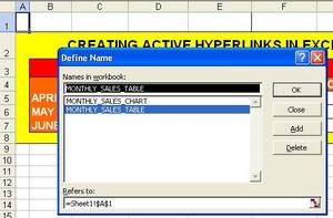
This will bring up a small popup screen that allows you to choose where you want the definition and what you want to call it. Click below to view the popup.
Click Here to view.
On the popup window you will notice that the location is already chosen by where selected earlier (on the bottom left of where your chart is). Now you have to name it. To name it simply choose a descriptive term like Sales_Chart where there are no spaces at all. You can use an underscore as a separator but no hyphens or spaces.
Once this is done you click the Add button which will bring the name into the center section of the table. Then you can just click OK. This defined your first location on the chart. Now you can link from any text to that area.
Creating a Link to the Defined Name
Right click on the title header of the table you created. In my case it says Monthly Sales Figures. Scroll down to Hyperlink and click on it. Click on the link below to view an example
Click Here to view.
Once the next page pops up you will have several choices to determine how you want the link to act. Click on the link below for an example of this pop up screen.
Click Here to view.
Once this screen pops up be sure to choose to link to a place in this document. Once you click there (on the left) it will bring up a list of possible choices on the right which at this point shouldn’t be very many, probably one. Choose the correct link you set up previously and click OK.
As soon as you do this you’ll notice that the text on the link has been unformatted. You can fix this by redoing it to the way you had it including changing the size, font, bold, and color. Once you do this you should be able to click on it and the link will take you right to the chart.
Linking back to the table
Now we want to be able to link back to the original table. This comes in extremely handy if you have multiple tables and multiple charts. First, lets define another name.
Defining the Second Name
Since your table is most likely at the very top of the page, I recommend highlighting A1 or the first cell. Once you choose which cell to highlight click on “Insert” then go down to “Name” then over to “Define” just as before. This time choose a similar name but call it table instead of chart. I chose “Monthly_Sales_Table”. Click on the link below to see the example.
Click Here to view.
Creating a Link at the Chart back to the Table
To link back to the table, first we need some text to link from. I always choose to create a nice bold link to the side of the chart. I highlighted 4 cells adjacent to the center of the chart and merged them by clicking on the merge and center tool to the right of the center right and left justify buttons. This makes it one large cell.
Once I have chosen the cell, I typed “Back to Table” in the cell. I then right clicked on it and choose Format Cell and choose the alignment tab with center and center as the choices and clicked OK.
Then I formatted the text by making the text 14 bold white and the background red. I also chose to outline the cell by clicking on the Outline button next to the hyperlink button on the toolbar and chose all 4 sides. Click on the link below to view my formatted cell.
Click Here to view.
Once that was finished, I then right clicked on the cell and chose insert hyperlink and went through the same steps as before only this time I chose the new link, “Monthly_Sales_Table”. Click on the link below to view the example.
Click Here to view.
Be sure to choose in this document and the new link you just created and click OK. Once you do this you’ll have to reformat the text back to the way it was but it is worth it. The other option is to not format it until after you are finished with the link but either way is fine, I just like to see what it will look like.
Once you finish reformatting the link you should be able to click back and forth on these links until you turn blue in the face. Now the real beauty of this trick may not be apparent but when you have a project that involves 25 separate tables you will be thankful that you have read this, it will make it much more manageable because you can click back and forth on the links and the person you are creating the charts for will be very pleased with you.
Good Luck – Vince Pendley


")